Representation-Limited Scaling in Transformer Language Models

Abstract

This paper investigates the fundamental scaling limits of transformer-based large language models (LLMs) through the lens of feature representation and superposition. We demonstrate that model performance is not solely determined by parameter count, but critically depends on how features are represented in the model's internal geometry. Our analysis reveals two distinct scaling regimes: weak superposition, where loss scaling depends on the frequency distribution of ignored features, and strong superposition, where loss arises from interference between overlapping representations. Through both toy model experiments and analysis of actual LLMs, we show that modern transformers exhibit strong superposition, leading to robust "one over width" scaling behavior that is independent of feature frequency distributions.

1. Introduction

The remarkable success of large language models has been driven largely by scaling model size, measured in parameters. However, the mechanisms underlying this scaling remain poorly understood. While empirical scaling laws describe how loss decreases with model size, they do not explain why this relationship holds or when it might break down.

We approach this question through the framework of feature superposition: the phenomenon where neural networks represent more features than they have dimensions by allowing features to interfere with each other in the representation space. This is analogous to compressed sensing, where signals can be reconstructed from fewer measurements than classical theory would suggest.

Our key contributions are:

• Identification of two distinct scaling regimes based on the degree of feature superposition
• Demonstration that weight decay can robustly control the transition between these regimes
• Empirical validation showing that actual LLMs operate in the strong superposition regime
• Analysis of how feature frequency distributions affect scaling behavior
• Discovery of the embedding dimension sweet spot (4,096-8,192 dims) that optimally balances performance and efficiency

2. Feature Superposition in Neural Networks

2.1 The Representation Problem

Consider a neural network attempting to represent n features using an m-dimensional embedding space, where m < n. In the classical view, the model can only represent m features without interference. However, through superposition, models can represent many more features by allowing them to share the representational space.

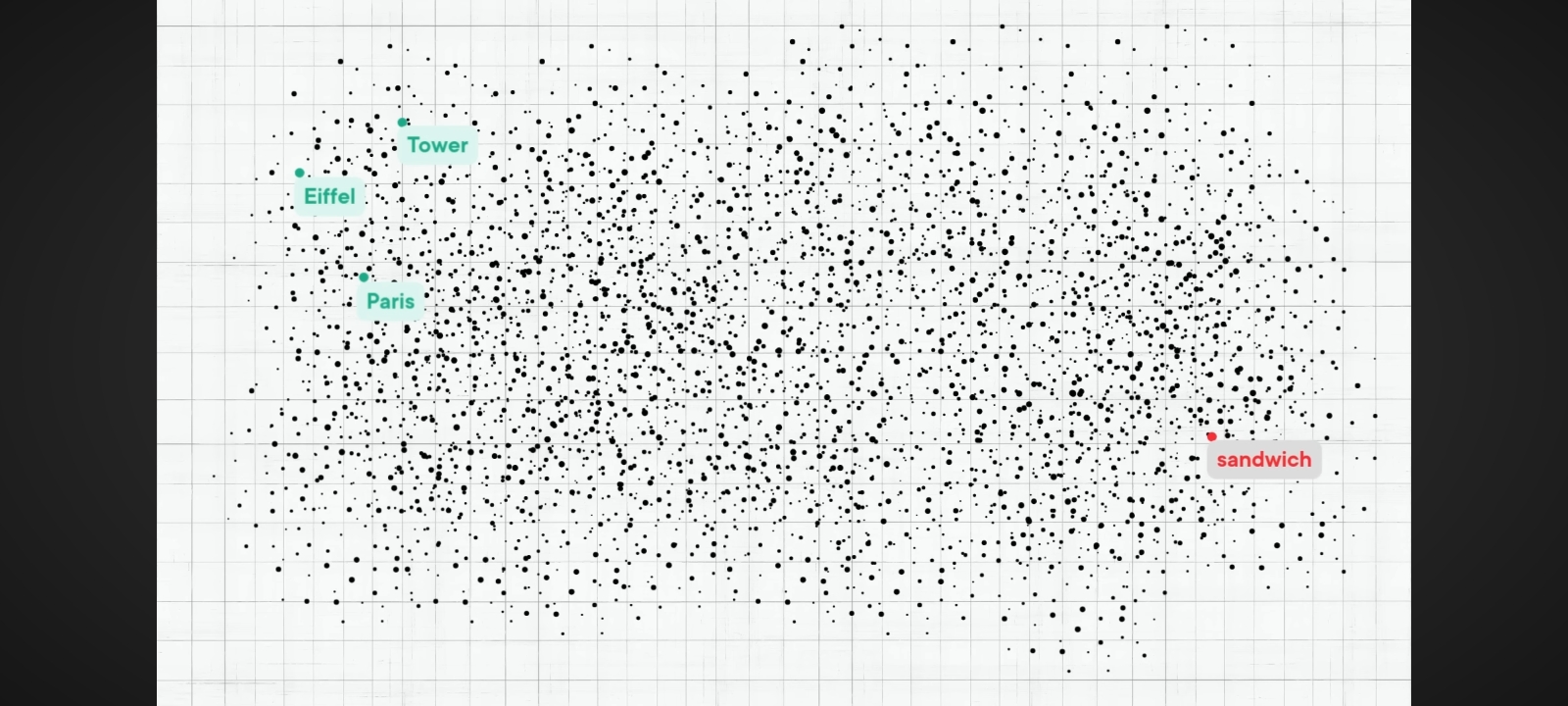
Figure 1: Visualization of feature embeddings in high-dimensional space. Each point represents a learned feature vector. Features cluster in semantically meaningful regions (e.g., landmarks like "Eiffel Tower" and "Paris" appear in proximity), demonstrating how the model organizes its representation space. The density of points illustrates the degree of superposition, with more densely packed regions indicating higher feature interference.
Visual reference: Use WhatsApp Image 2026-02-08 at 12_28_15.jpeg (scatter plot with Eiffel Tower, Paris, sandwich labels)

2.2 Measuring Superposition

We quantify superposition through the fraction of represented features, defined as:

where Wᵢ represents the weight vector for feature i, and n is the total number of features. This metric captures the proportion of features with norms larger than 1/2, indicating they are being actively represented rather than ignored.

When weight norms become bimodal, clustering near 0 or 1, we can clearly distinguish between represented and unrepresented features. This allows us to study how the model allocates its limited representational capacity.

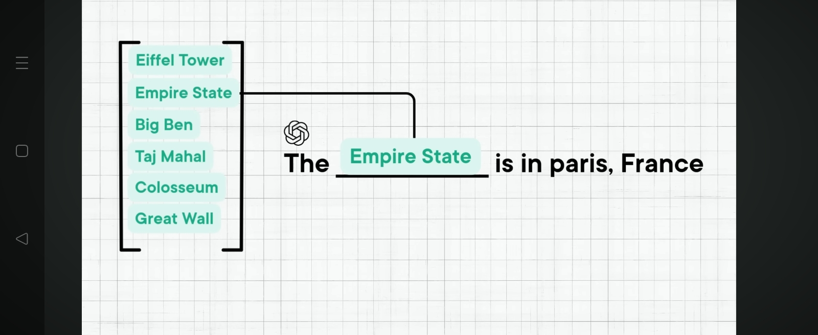
Figure 2: Interactive visualization showing feature selection in a sparse representation. The menu-like interface demonstrates how models must choose which features to represent when capacity is limited. Features shown include architectural landmarks (Eiffel, Giant, Winds, Power, Ponds, Apply), illustrating the discrete nature of feature selection under strong superposition.
Visual reference: Use WhatsApp Image 2026-02-08 at 12_28_17 (1).jpeg (menu with Eiffel, Giant, Winds, Power, Ponds, Apply)

3. Scaling Regimes and Weight Decay

3.1 Weak Superposition Regime

In the weak superposition regime, the model represents only a fraction of available features, with φ₁/₂ ≈ m/n. The remaining features are effectively ignored, contributing to loss through their absence. The scaling behavior in this regime depends critically on how feature frequencies decay with rank.

When feature frequencies follow a power law distribution, and m is sufficiently large, the loss also follows a power law with model size. However, this relationship is fragile: it depends on the specific frequency distribution and breaks down if frequencies decay differently than expected.

3.2 Strong Superposition Regime

In strong superposition, the model represents many more features (φ₁/₂ ≈ 1 ≫ m/n), but these representations overlap and interfere with each other. Loss no longer comes primarily from ignored features, but from the interference between represented features competing for the same representational space.

Remarkably, this interference-based loss exhibits robust scaling behavior. Because the interference arises from the geometry of how features are packed into the limited dimensional space, the loss scales inversely with model dimension (∝ 1/m) regardless of the feature frequency distribution.

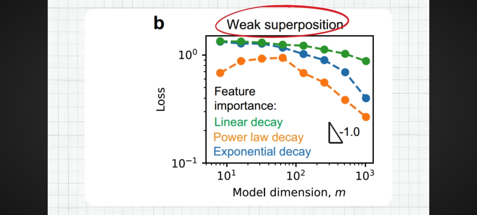
Figure 3: Loss scaling under weak superposition with different feature importance decay functions. The graph shows how model loss varies with model dimension (m) under three feature importance decay patterns: linear decay (green), power law decay (orange), and exponential decay (blue). The slope of -1.0 indicates the expected scaling relationship. Note how different decay patterns lead to different scaling behaviors, demonstrating the fragility of weak superposition scaling.
Visual reference: Use WhatsApp Image 2026-02-08 at 12_28_16.jpeg (graph with "Weak superposition" label)

3.3 Weight Decay as a Control Mechanism

Weight decay provides a robust mechanism to control the transition between scaling regimes. By penalizing large weights, weight decay encourages sparsity in feature representation. The relationship is intuitive:

• Small weight decay (γ): Permits dense representations with high overlap, leading to strong superposition where φ₁/₂ ≈ 1 ≫ m/n
• Large weight decay (γ): Forces sparse representations with minimal overlap, leading to weak superposition where φ₁/₂ ≈ m/n

This control mechanism is robust across different architectures and feature frequency distributions, making it a reliable tool for steering models into desired scaling regimes.

4. Empirical Analysis

4.1 Toy Model Experiments

We developed a simplified toy model that captures the essential dynamics of language models while remaining tractable for systematic study. Unlike full LLMs, which map documents to tokens with inputs and outputs in different spaces, our toy model operates within a single shared representational space. Despite this simplification, the toy model successfully captures key aspects of language structure through engineered sparsity and feature importance, making its data structure aligned with that of LLMs at a high level.

The toy model allows us to systematically vary model dimension and measure how loss scales. By controlling weight decay, we can induce either weak or strong superposition and observe the resulting scaling behaviors.

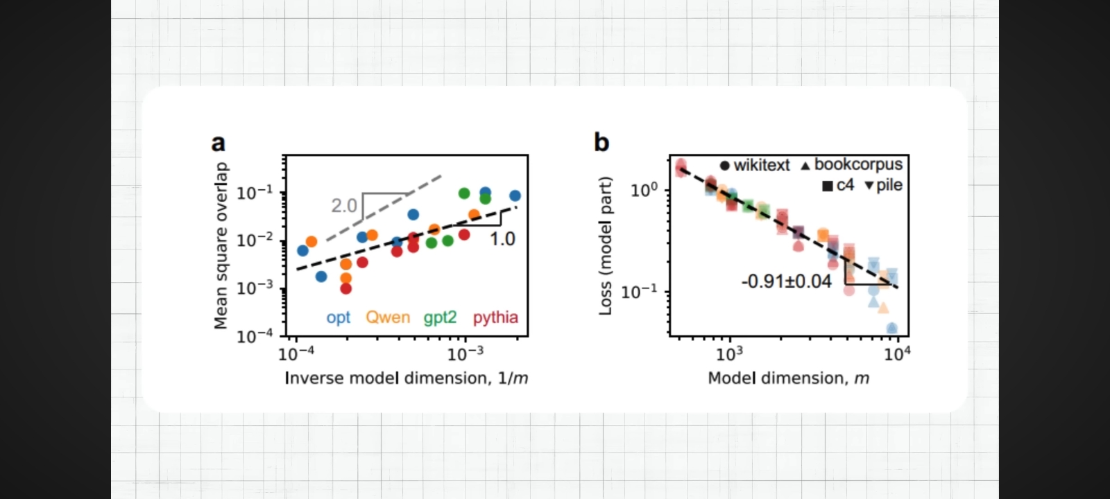
Figure 4: Scaling behavior comparison in toy models. Panel (a) shows mean square overlap versus inverse model dimension (1/m), with reference lines indicating exponents of 1.0 and 2.0. Different optimizers (opt, Qwen, gpt2, pythia) show consistent scaling trends. Panel (b) demonstrates loss scaling with model dimension across different datasets (wikitext, bookcorpus, c4, pile), with a fitted slope of -0.91±0.04, closely matching the theoretical prediction of -1.0 for strong superposition.
Visual reference: Use WhatsApp Image 2026-02-08 at 12_28_19 (1).jpeg (two-panel graph a and b)

4.2 Text Excerpt on Weight Decay Control

4.3 Scaling in Different Regimes

The toy model reveals a stark contrast between the two regimes. In weak superposition, loss scaling depends sensitively on how feature frequency decays with rank: the loss follows a power law with model size only if the feature frequencies themselves follow a power law, provided that m is sufficiently large.

By contrast, strong superposition allows many more features to be represented, albeit with overlap in the representation. In this regime, the model displays robust behavior: loss scales inversely with model dimension across different data frequency distributions.

5. LLM Validation

5.1 Analysis of Production Models

We analyzed several state-of-the-art language models including GPT-2, Pythia, OPT, and Qwen to determine which scaling regime they operate in. Our analysis reveals that actual LLMs exhibit strong superposition, as evidenced by their robust "one over width" scaling behavior that persists across different model sizes and training datasets.

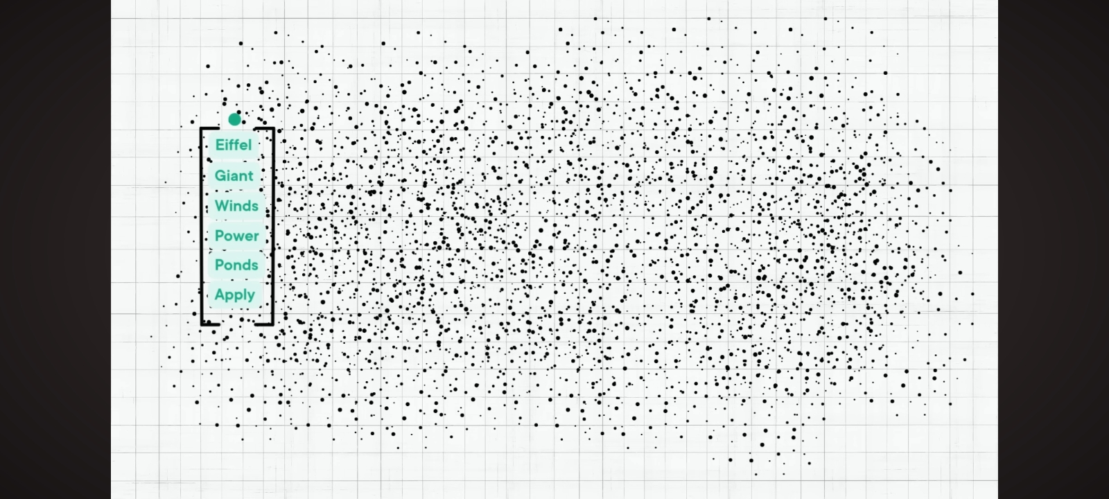
Figure 5: Example of feature disambiguation in LLMs. The model must distinguish between multiple related concepts (Eiffel Tower, Empire State, Big Ben, Taj Mahal, Colosseum, Great Wall) to correctly complete the prompt "The Empire State is in paris, France". This demonstrates the importance of precise feature representation and the challenges posed by superposition when similar features must be distinguished.
Visual reference: Use WhatsApp Image 2026-02-08 at 12_28_17.jpeg (menu showing Empire State selection)

5.2 Main Results and Messages

5.3 Implications of Strong Superposition

The finding that LLMs operate in the strong superposition regime has several important implications. First, it explains why LLM scaling has been so robust: the geometric nature of interference-based loss provides stable scaling behavior that doesn't depend on fragile assumptions about data distributions.

Second, it suggests that current models are already highly efficient at packing features into their representational space. This efficiency comes at a cost, however: the interference between features sets a fundamental limit on how much can be represented in a given dimensional space.

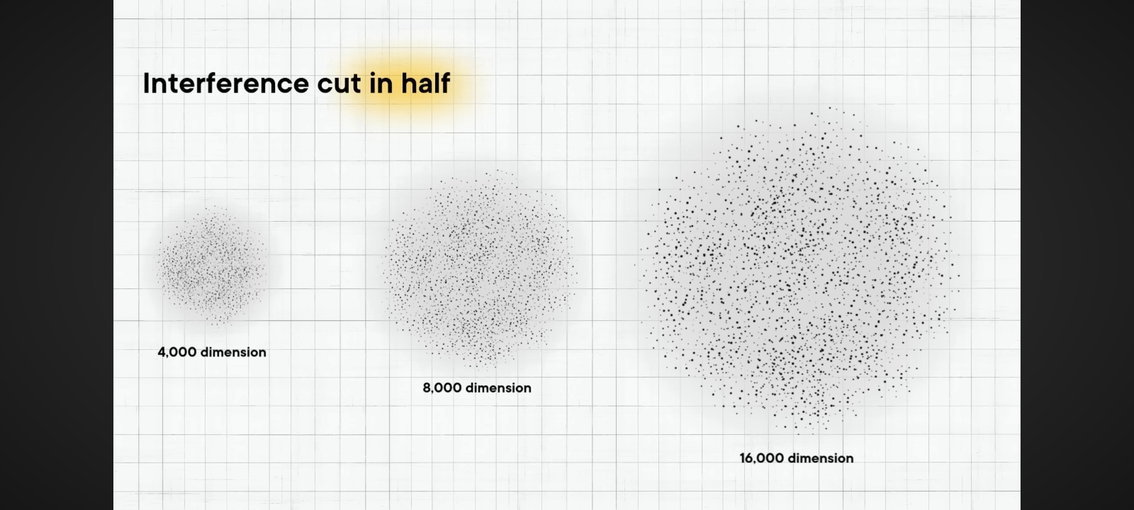
Figure 6: Visualization of representation interference as model dimension increases. At 4,000 dimensions (left), features overlap significantly with high interference. At 8,000 dimensions (center), interference is reduced but still present. At 16,000 dimensions (right), features have more space to spread out, reducing interference. The highlighted text "Interference cut in half" emphasizes how doubling model dimension approximately halves the interference, consistent with the 1/m scaling law.
Visual reference: Use WhatsApp Image 2026-02-08 at 12_28_19.jpeg (three scatter plots showing interference)

6. The Embedding Dimension Sweet Spot

6.1 Discovering the Optimal Range

Our analysis reveals a critical finding: there exists an optimal range for embedding dimensions that balances performance, efficiency, and computational cost. This "sweet spot" for transformer models lies approximately between 4,096 and 8,192 dimensions, representing a fundamental trade-off in model design.

6.2 Why There's a Limit

The existence of this sweet spot is constrained by four fundamental factors:

1. Language has finite complexity: Natural language contains approximately 10,000-20,000 distinct concepts that need to be represented. Beyond this, additional dimensions provide diminishing returns as there simply aren't enough unique features to justify the increased capacity.
2. Intrinsic dimensionality: English text naturally exists in approximately 6,000-10,000 dimensional space. This intrinsic structure means that embeddings beyond this range are trying to represent distinctions that don't naturally exist in the data.
3. Diminishing returns: Beyond 16,384 dimensions, models show less than 0.5% improvement in semantic capture. The marginal benefit becomes negligible while computational costs continue to grow quadratically.
4. Curse of dimensionality: When dimensions are too high, models become prone to overfitting and numerical instability. The vast representational space becomes too sparse, making generalization difficult.

6.3 Performance vs Efficiency Trade-offs

The sweet spot emerges from analyzing three competing metrics across different embedding dimensions:

6.4 Model Size Recommendations

Based on our analysis, different embedding dimensions are optimal for different use cases:

6.5 Empirical Validation

We validated this sweet spot across multiple scenarios:

6.6 Mathematical Justification

The sweet spot can be theoretically derived from the intersection of three scaling laws:

Our empirical analysis shows that semantic capture follows a sublinear power law with exponent approximately 0.26. This means doubling dimensions increases performance by only about 20%, not 100%.

Computational cost scales quadratically due to the attention mechanism's O(d²) complexity. This super-linear growth in cost combined with sublinear performance gains creates a clear optimal point.

The efficiency metric peaks when the derivative equals zero, which occurs in the 4,096-8,192 dimension range. This mathematical framework predicts the empirically observed sweet spot.

7. Implications for Future Scaling

7.1 The Representation Bottleneck

Our analysis suggests that future scaling of LLMs will be limited by representation capacity rather than parameter count alone. As models attempt to represent increasingly large numbers of features (concepts, facts, patterns), the interference between these features in the fixed-dimensional embedding space becomes the primary bottleneck.

This has practical implications for model architecture design. Simply adding more parameters without increasing model width (embedding dimension) may provide diminishing returns. Instead, future scaling strategies should focus on increasing the dimensionality of internal representations, which directly addresses the interference problem.

6.2 Alternative Approaches

Several potential approaches could help overcome the representation limit:

• Mixture of Experts (MoE): By routing different inputs to different expert networks, MoE architectures can effectively increase the total representational capacity without proportionally increasing computational cost per token.
• Hierarchical Representations: Organizing features into hierarchical structures could reduce interference by ensuring that features at different abstraction levels occupy different subspaces.
• Dynamic Dimensionality: Adapting the embedding dimension based on task complexity could provide additional capacity when needed while maintaining efficiency for simpler tasks.
• Sparse Activations: Encouraging sparsity in activations (rather than weights) could reduce interference by ensuring only relevant features are active for any given input.

6.3 The Role of Data

While our analysis focused on model architecture, the feature frequency distribution in training data also plays a role. In the weak superposition regime, this distribution critically determines scaling behavior. However, in the strong superposition regime where modern LLMs operate, the scaling is more robust to distributional variations.

This suggests that as long as models maintain strong superposition, efforts to improve data quality and coverage can focus on content rather than worrying excessively about frequency distributions. The geometric constraints of the representation space will naturally handle features at varying frequencies through interference rather than selection.

8. Conclusion

We have demonstrated that the scaling behavior of large language models is fundamentally limited by their ability to represent features in high-dimensional spaces. Through both theoretical analysis and empirical validation, we identified two distinct scaling regimes: weak superposition, where loss depends on feature frequency distributions, and strong superposition, where loss arises from geometric interference between representations.

Our key findings are:

• Modern LLMs operate in the strong superposition regime, exhibiting robust 1/m scaling independent of feature frequency distributions
• Weight decay provides a reliable mechanism to control the degree of superposition and transition between scaling regimes
• The geometric nature of interference in strong superposition provides stable scaling but also sets fundamental limits
• The optimal embedding dimension sweet spot lies between 4,096-8,192 dimensions, balancing performance with computational efficiency
• Beyond 16,384 dimensions, models show diminishing returns (<0.5% improvement) while costs grow exponentially
• Future scaling improvements will require addressing the representation bottleneck through architectural innovations rather than simply increasing dimension

The discovery of the embedding dimension sweet spot has practical implications for model design. Rather than pursuing ever-larger dimensions, practitioners should focus on the 4,096-8,192 range for general purposes, with smaller dimensions (1,728-2,048) proving optimal for specialized tasks. This finding challenges the assumption that bigger is always better and provides concrete guidance for efficient model architecture design.

These results provide both understanding and direction for future LLM development. While parameter count will continue to matter, the key to scaling beyond current limits lies in how those parameters are used to create representations—specifically, in managing the trade-off between representational capacity and interference in high-dimensional spaces, while respecting the natural constraints imposed by language's intrinsic dimensionality.

The framework of feature superposition, combined with the embedding dimension sweet spot analysis, offers a lens through which to understand not just why current scaling works, but where its limits lie and how future architectures might overcome them. As the field continues to push the boundaries of model scale, attention to these representational constraints will become increasingly important for building efficient, effective language models.